Theory of Light and Color

38. Key Points
When Evaluating the Optical Characteristics of LEDs (Part 1)
Since the invention of the red LED in the early 1960s, development has continued for other monochromatic LEDs such as yellow, orange, and yellow-green, and these LEDs have become widespread through use in displays. In the early 1990s, the blue LED was developed and brought to market, which made it possible to create white LEDs to be used in general lighting as well.
At first, white LEDs had many issues, such as poor color rendering, especially compared to traditional light sources like incandescent bulbs and fluorescent lamps. However, rapid technological advances solved many of these problems, and they were quickly adopted due to advantages such as energy efficiency, long life, high brightness, and compact size. While white LEDs continue to replace traditional light sources, monochromatic LEDs continue to have many applications. Whether a monochromatic LED or a white LED, optical characteristics need to be measured and evaluated based on how it will be used.
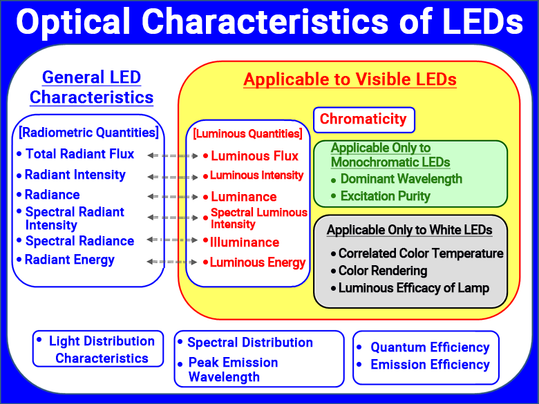
That said, "optical characteristics of LEDs" encompasses a lot, as shown on the right. Among these, the characteristics in the yellow box apply to all LEDs that emit light in the visible spectrum. Of those, the characteristics in the green box apply only to monochromatic LEDs, and those in the gray box are unique to white LEDs.
When measuring, evaluating, or interpreting these optical characteristics, there are differences compared to traditional light sources. If you try to measure LEDs in the same way as traditional sources, the results may vary more than expected.
It is important to keep these unique differentiators in mind when testing LEDs and to take different precautions than you would for conventional light sources. Because LEDs have features that older light sources did not, you can get the best performance out of them by understanding and managing these unique LED characteristics covered below and using them appropriately for the intended application.
(1) Variability in Luminous Intensity Measurements
To measure the optical properties of a light source, such as radiant and luminous quantities, you must set up the detector according to its defined optical requirements. Then, you must use a properly calibrated measuring device.
For example, to measure luminous intensity (light output per unit solid angle), you point a lux meter directly at the light source from a distance of d [m], and measure the illuminance E [lx = lm/m2] of the light emitted within a narrow solid angle.
You then calculate the luminous intensity I [cd = lm/sr] in that direction using the formula:
I = E·d2 ≪1≫
So, when measuring luminous intensity, parameters such as the distance and the area of the sensor that collects the light (the lux meter's detection surface) must be carefully controlled. However, when several LED manufacturers ran a round robin test (a shared measurement test) over ten years ago using the same LED sample and agreed-upon conditions, the results still varied by several tens of percent. ≪2≫
With traditional light sources, the variation in results from round robin testing usually stayed within a few percent. In theory, the methods for measuring radiant and luminous quantities should apply equally to LEDs and traditional light sources. But in practice, measurements of LEDs tend to show more variability. This is largely due to the unique features of LED light sources.
One major reason is the extremely small size of LED light sources compared to traditional ones. LEDs are tiny solid-state semiconductor light emitters. Many of them have light-emitting surfaces smaller than 1 mm2, which is much smaller than typical light sources. LEDs can be used in many forms, such as packaged components or as bare chips mounted directly to circuit boards.
Because of this small size, applying the same measurement conditions used for traditional light sources to LEDs often leads to significantly more variability in measurement results, even if you think you are measuring them in the same way.
(2) Issues Related to Optical "Axes"
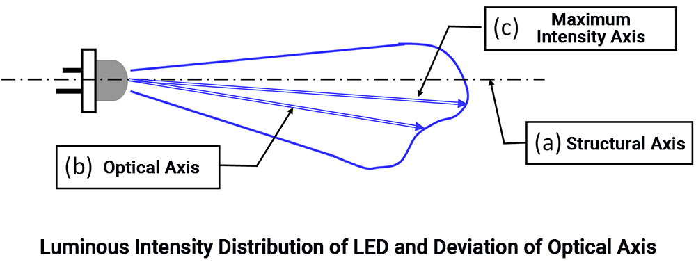
When measuring how much light is emitted in a given direction from a light source, we deal with a property called luminous intensity distribution. There are generally three types of optical axes to consider:
(a) Structural axis: the mechanical axis determined by the structure of the LED package
(b) Optical axis: the center direction of the light distribution pattern
(c) Maximum luminous intensity axis: the direction in which the luminous intensity is strongest
For traditional light sources like incandescent bulbs (which generally emit light evenly in all directions except at the base) or fluorescent lamps (which have a uniformly diffused emission from the tube surface), the light distribution is broad and smooth. In these cases, the three types of axes listed above usually align well. However, it is quite common for these three axes to be noticeably misaligned in the case of LEDs mounted in packages.
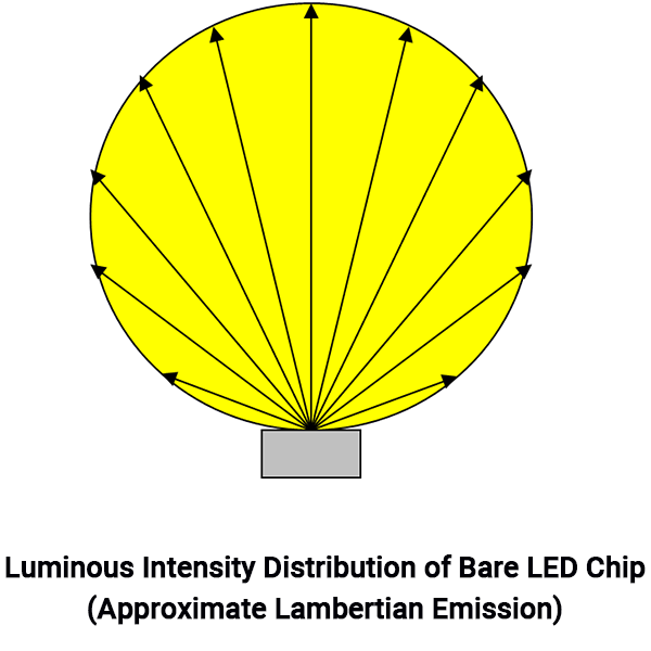
Light emitted directly from a bare LED chip tends to have a fairly even, diffused distribution pattern (as shown in the figure on the right). But once the LED is packaged, additional components such as focusing lenses or reflectors are often added to improve light efficiency and produce a more directional beam, typically aimed forward. This is common in "bullet-type" LED packages.
When mounting the LED chip into the package, any slight misalignment in its structural or positional placement can cause significant variation in the light distribution.
Ideally, the LED chip should be mounted symmetrically along the mechanical axis of the package, especially when a lens or reflector is used. But in reality, even a tiny shift from this ideal axis can cause the direction of emitted light to change noticeably. If the LED has a wide light distribution pattern, then small positioning errors have less effect. But the more focused the light is, the greater the shift between the structural axis and the actual optical axis tends to be. This also causes the symmetry of the light distribution to break down, leading to differences between the optical axis and the maximum luminous intensity axis.
Because of this, when measuring luminous intensity from LEDs with narrow distribution angles, even small changes in the size or placement of the sensor detection area (such as its distance from or angle to the LED) can cause big differences in the measured values. This makes measurement results prone to fluctuation. If you try to remeasure the same sample LED at a different time, it may be difficult to replicate the same measurement conditions, which can lead to inconsistencies and poor reproducibility of results.
(3) CIE Averaged LED Intensity
Setting a wider measurement solid angle (field of view) can help average out sharp changes in light distribution or axis misalignment to reduce measurement variation in LED luminous intensity.
Based on this idea, the CIE (International Commission on Illumination) established a measurement standard known as CIE Averaged LED Intensity (ILED).
This standard defines two types of measurement conditions, depending on the size of the measurement solid angle (Ω):
• Condition A: Ω = 0.001 steradians
• Condition B: Ω = 0.01 steradians
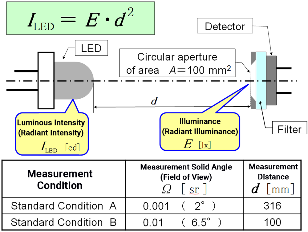
For both Conditions A and B, the sensor (an illuminance meter or radiometer) uses a fixed circular detection area of 100 mm2 (with a radius of about 5.64 mm).
The measurement distance is set to:
• Condition A: d = 316 mm
• Condition B: d = 100 mm
These settings determine the measurement solid angle (field of view) for each condition.
(4) Challenges with CIE Averaged LED Intensity
The introduction of CIE Averaged LED Intensity (ILED) has significantly reduced variation in LED intensity measurements compared to before. However, it has not completely solved all the problems. There are still several ongoing challenges:
[1] Issue with Measurement Distance
In the standard, the reference position on the light source side is defined as the tip of the LED package, even though the actual LED chip is mounted inside the package. In packages that use lenses or reflectors, the actual light-emitting position differs from the optical emission point. But because that position is not clearly defined, the easily identifiable tip of the package is used as the reference point for measurement distance.
On the illuminance meter side, the reference distance is defined as the frontmost surface of the sensor. However, in many cases, there are optical filters or other components between the aperture surface and the actual sensor surface, meaning the true light-receiving position is slightly farther back.
If the measurement distance is large enough, small differences in these reference positions on both the light source and detector sides can be ignored. But if the distance is short, these offsets can affect measurement accuracy. In Condition B, where the measurement distance d is short, this becomes a bigger source of variation.
[2] Issue with Color Mismatch Errors (Chromatic Photometric Errors)
Monochromatic LEDs have a narrow spectral distribution. When evaluated using the standard luminous efficiency curve V(λ), any difference between the actual spectral sensitivity of the sensor and the theoretical ideal can directly lead to a measurement error known as chromatic photometric error.
In the CIE Averaged LED Intensity standard, the allowed error in the spectral response of the illuminance meter is defined as the integrated error over the entire visible spectrum compared to V(λ). Since V(λ) has both positive and negative error regions depending on the wavelength, broad-spectrum sources like white LEDs tend to average these out and reduce the overall error.
However, if the emission spectrum of a monochromatic light source falls in a wavelength region where the sensitivity error is high, chromatic photometric errors can become significant.
This is especially important when using a filter-type sensor instead of a spectral-type sensor. LEDs such as blue, yellow, or red, which emit in those sensitive ranges, are more prone to this type of error. Even with white LEDs, especially the Blue-YAG type (which includes strong blue light for exciting the phosphor), chromatic photometric errors are more likely to appear.
[3] Stabilization of LED Output During Operation
As described in the next section, when an LED is powered on, the temperature of the semiconductor junction rises. This causes the emission wavelength to shift toward longer wavelengths. To avoid errors from this shift, it's important to either wait until the LED reaches a stable emission state (thermal equilibrium) or carefully control the timing between powering the LED and taking the measurement.
(5) Shift in Emission Wavelength (Spectral Distribution and Peak Wavelength) Due to Junction Temperature Rise
Spectral distribution is one of the most important fundamental characteristics of a light source. It is extremely important to measure the spectral distribution correctly and evaluate it based on the intended use.
Regardless of the type of light source, supplying power to generate light causes heat. The amount of heat generated varies widely depending on the type, from high-heat incandescent bulbs to lower-heat luminescent sources such as fluorescent lamps and LEDs.
While LED light sources generate relatively little heat, they still heat up when powered. This causes the temperature of the LED chip (semiconductor junction) to rise. As the junction temperature rises, the energy conversion efficiency drops, leading to a slight decrease in emission output (radiant flux). More importantly, the emission wavelength (spectral distribution) shifts to a longer wavelength as the junction heats up. Even when used within the rated current, the shift can quickly reach about 5 nm.
The figure below simulates changes in luminous quantities (i.e., perceived brightness) for three types of monochromatic LEDs (blue, green, and red), assuming a 5 nm redshift in emission wavelength caused by junction temperature rise immediately after powering on. Although actual heating would slightly lower total light output, this simulation assumes it stays constant to isolate the effect of wavelength shift. Since the emission wavelength ranges of blue and red LEDs fall in areas of the spectrum where the standard luminous efficiency curve V(λ) changes rapidly, a small shift greatly affects the measured brightness.
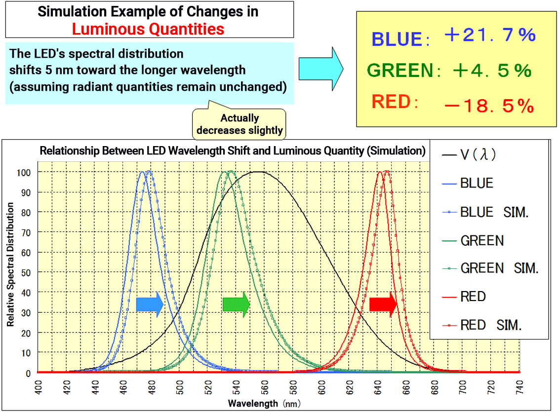
The simulation results show:
• Blue LED: luminous flux increases by about 22%
• Red LED: luminous flux decreases by about 19%
• Green LED: luminous flux increases by about 5%
The impact is less drastic for the green LED because its emission wavelength is in a part of the spectrum where V(λ) changes more gradually. While the simulation assumes no drop in radiant output, there would be a slight decrease in real conditions. So roughly speaking, a 5 nm wavelength shift causes a 20% increase for blue LEDs and a 20% decrease for red LEDs in luminous flux. Shifts larger than 5 nm are not unusual, so deviations over ±20% often occur.
This simulation focused on luminous flux using the standard luminous efficiency function V(λ). However, when measuring light color (chromaticity), the evaluation function changes to the  color matching functions.
The  function in particular is steeper than V(λ), so a shift in emission wavelength can cause significant fluctuation in stimulus value Z and measurements of blue LEDs. As for how the emission wavelength shift progresses over time, the junction temperature rises gradually after turning on, which slowly shifts the emission wavelength to the longer side until it stabilizes at thermal equilibrium. To get stable measurements, it is best to wait until the LED reaches this equilibrium state.
That said, LEDs are not always used in thermal equilibrium in real applications. So, it may be necessary to measure and evaluate LED performance under actual usage conditions, such as drive current and the timing of light use after power-on.
Since the temperature of the junction changes significantly right after power-on, if precise evaluation is needed, an electronic timer can be used to set the measurement timing instead of measuring by hand. Depending on whether the performance of the LED is more important immediately after turning on or in a stabilized state, you need to carefully choose the timing for your measurements.
It is also a good idea to collect correlation data between measurements taken during thermal equilibrium and those taken under real-use conditions. This is especially true for high-power LEDs, which generate more heat and are more affected by junction temperature changes.
Finally, when evaluating radiant flux, the effect of wavelength shift on measurement is considered minimal, since the spectral sensitivity of the measuring instrument is fixed. However, there will still be a decrease in energy conversion efficiency due to heating.
In this section, we focused on two major causes of variation in LED measurement results: (1) the misalignment of three types of optical axes, and (2) spectral distribution shifts due to junction temperature rise. In the next part, we will look at additional contributing factors.
Comment
≪1≫ Calculating luminous intensity from illuminance measurements
Luminous intensity is measured by using the illuminance E [lx] at a certain distance d [m] from the light source, based on the luminous flux φ [lm] emitted within the solid angle Ω [sr] which is determined by the detector's receiving area S [m2] and the distance d [m]:
Ω = S / d2
If the measured illuminance is E [lx] = φ / S [lm / m2] then the luminous flux emitted within the solid angle is:
φ [lm] = E [lx]·S [m2]
Therefore, the luminous intensity I [cd] of the light source is calculated as:
I [cd] ≡ φ / Ω [lm / sr] = (E·S) / (S / d2) = E·d2
≪2≫ Data on variation in round-robin test results
For example, a round-robin test conducted by seven Japanese LED manufacturers using actual products showed variability in measurement results.
(2000 Illuminating Engineering Institute of Japan 33rd National Convention Presentation Material S-6)