Theory of Light and Color

26. Color Difference and Uniform Color Space
Color difference between two colors is another consideration for color systems. The Munsell color system is a simple method for evaluating color tolerance by visual comparison. However, it can fall short in situations that require objective, quantitative evaluation. (Please refer to Comment ≪2≫ in Chapter 21). In such cases, there are numerical expressions for color difference.
(1) The MacAdam Ellipse and Color Difference Non-Uniformity
The distance between two points on the chromaticity diagram indicates the color difference between them.
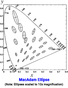
The figure on the right shows MacAdam ellipses on the xy chromaticity diagram (≪7-1≫ developed by David MacAdam in the United States in 1942). The ellipses indicate the range of color differences indistinguishable to the naked eye for various colors (chromaticity points). The different sizes show how the display of color difference on the xy chromaticity diagram lacks uniformity. Please note that the scale of the ellipses is magnified 10 times their actual size.
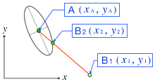
Consider color A in one ellipse with the coordinates (xA, yA) at the center of the ellipse (the intersection of the major and minor axes) and color B at a chromaticity point different from A. If the chromaticity coordinate of color B is far outside the ellipse at B1 (x1, y1), you can see they are different colors. However, as B gets closer to A, both shades become similar. If B is on the boundary of the ellipse or inside it, such as B2 (x2, y2), the two colors are indistinguishable to the naked eye. The MacAdam ellipse defines the boundary where colors A and B become indistinguishable.
The ellipses shown in the xy chromaticity diagram vary in size depending on their position. They are larger in the upper region (green area) and smaller in the lower left (blue to bluish-purple area). In other words, depending on the color (position on the chromaticity diagram), the distance on the chromaticity diagram is inconsistent with the naked eye’s sense of color difference (unequal spacing in color difference)
Even if the distance between two colors on the chromaticity diagram is the same, the difference can be distinguished in the blue region (outside the color discrimination ellipse) but not the green region (inside the ellipse). Furthermore, the elliptical shape of the discrimination area is another indicator that the sense of color difference does not correspond to distance on the chromaticity diagram.
Therefore, when the color difference is expressed by the distance between the chromaticity points, it becomes extremely troublesome because the type of color and the direction of the color shift must be specified. The XYZ color system is an objective and quantitative system backed by scientific theory and experiments and an overall excellent system for displaying colors in very fine detail, but its biggest flaw is its representation of color difference. ≪1≫

(2) Improving Color Space Uniformity
If the distance between two points can match the color difference regardless of the color or the direction of color shift, a color system can objectively and quantitatively show uniform color shift. There have been multiple studies to improve color difference uniformity.
The CIE 1960 USC chromaticity diagram (uv chromaticity diagram) ≪2≫, CIE 1964 U*V*W* color space ≪3≫, and others were adopted and used in academic societies and industries. But these chromaticity diagrams and color spaces are still far from ideal despite their improved color difference uniformity. With continuous improvements, the CIE adopted two uniform color spaces in 1976, the CIE 1976 L*u*v* color space (CIELUV color space) and the CIE 1976 L*a*b* color space (CIELAB color space). In theory, only one should have been adopted. However, the two spaces are constructed from completely different ideas, and neither achieves the ideal uniform color space. As they have different advantages and disadvantages, it is hard to say which is better. As a result, both were adopted at the same time and have been widely used as basic uniform color spaces since 1976 despite their shortcomings. ≪4≫
(3) CIE 1976 L*u*v* Color Space (CIELUV Color Space)
The CIE 1976 L*u*v* color space was designed to address uniformity in color difference perception by modifying the CIE 1960 UCS (Uniform Chromaticity Scale) diagram. This adjustment involves stretching the v axis of the UCS diagram by 1.5 times, resulting in a new u’v’ chromaticity diagram to represent human visual perception of color differences more uniformly.
For object color, the color coordinates (L*, u*, v*) are defined by the following equations, calculated as relative values with respect to a perfect reflecting diffuser.
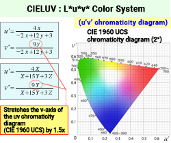
Y represents the stimulus value, and u’ and v’ represent the chromaticity of the object. Yn, u’n, and v’n represent the same values, respectively, for a perfect reflecting diffuser (standard white surface) under the same conditions. By setting the chromaticity of the standard white surface (white light source) as the origin (u*n, v*n) = (0, 0), the u*v* chromaticity coordinate is calculated using (u’, v’) and shows how much the color of the light reflected by an object changes when lit by white light. ≪6≫
This transformation ensures that the color difference perceived by the human eye is more uniformly represented across the entire color space. While a significant improvement compared to the MacAdam ellipses in the u’v’ chromaticity diagram and the uv chromaticity diagram ≪2≫, it is still far from the ideal uniform color space.
(4) CIE 1976 L*a*b* Color Space (CIELAB Color Space)
The CIE 1976 L*a*b* color space (CILAB color space) takes a completely different approach than the CIE 1976 L*u*v* color space (CIELUV color space) described above. The transformation formula defines a uniform color space for object color display in 3D Cartesian coordinates (L*a*b*):

X, Y, and Z are the tristimulus values of the sample object, and Xn, Yn, and Zn are those for the perfect reflecting diffuser (standard white surface). With this coordinate transformation, the a* and b* axes of the a*b* chromaticity diagram represent chromatic components; a* from green to red and b* from blue to yellow (see figure right). This arrangement setup mirrors the color opposites we naturally perceive.
Like the CIELUV color space, the a*b* chromaticity coordinate represents the chromaticity of the object color and uses the chromaticity of the standard white surface as the origin (a*, b*) = (0, 0). ≪6≫
The L* axis represents lightness in the same way it does in the CIELUV color space, but for the chromaticity a*b*, the tristimulus values are adjusted using a nonlinear operation to the power of 1/3 so the space reflects a uniform perception of color changes. You can think of it like a globe: L* is like the North and South Poles, showing how light or dark a color is, while a* and b* are like the longitude lines, showing the hue. And the a*b* chromaticity diagram is a flat slice through this color "world," helping us see how colors relate to each other in a way that makes sense to us.

(5) Calculation of color difference and its application to color shift inspection
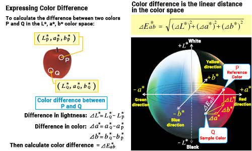
Multiple color differences between two colors can be represented by coordinate distance in a uniform color space. The following is an example of the CIE 1976 L*a*b* color space (CIELAB color space).
If the coordinate values of colors P and Q are P (L*P, a*P, b*P) and Q (L*Q, a*Q, b*Q) respectively, the distance between the coordinate points of both is the color difference ΔE*ab, and it can be calculated by the following formula.
(ΔL* = L*Q – L*P, Δa* = a*Q – a*P, Δb* = b*Q – b*P)
The color difference ΔE*uv in the CIE 1976 L*u*v* color space (CIELUV color space) can be calculated in the same way.
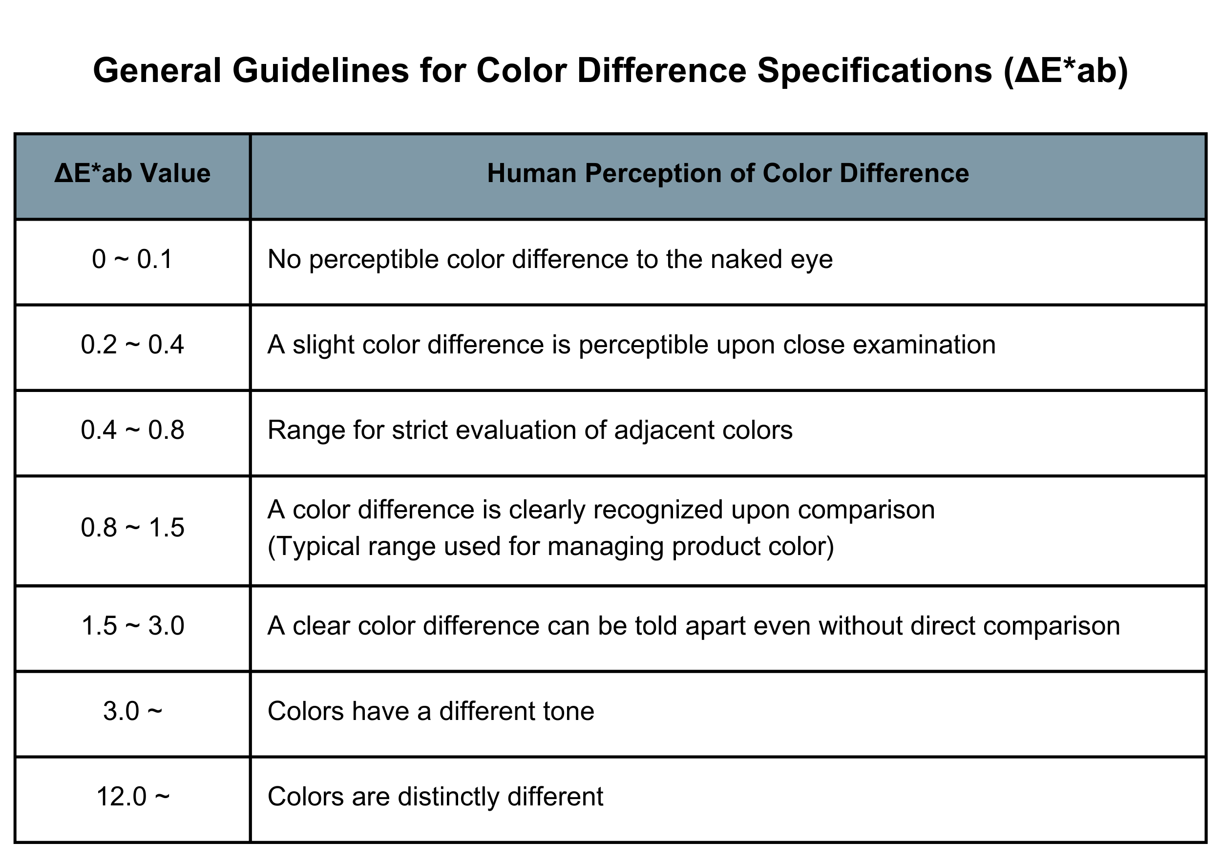
In the actual color shift inspection, you can obtain the colorimetric value of the reference color P (L*P, a*P, b*P) and that of the sample color Q (L*Q, a*Q, b*Q) using a colorimeter, and calculate color difference ΔE*ab from these colorimetric data, so you can perform stable inspection objectively, quantitatively, and for a long period of time.
The relationship between the value of ΔE*ab and the color difference with the naked eye is roughly as shown in the table below. It is a great advantage in practical use that precise color shift can be managed just by the value of ΔE*ab without specifying the color types.
Comment
≪1≫ The trade-off between additive color mixing compatibility and color difference uniformity
The xy chromaticity diagram (XYZ color system) has the significant advantage of being able to display colors with extremely fine precision in an objective and quantitative manner. And as described in Comment ≪5≫ of Chapter 21, it also has the benefit of being well-suited for additive color mixing. This compatibility with additive color mixing stems from the fact that the XYZ color system (or Yxy color system) is mathematically a linear space.
On the other hand, the L*a*b* color system sacrifices its compatibility with additive color mixing to improve color difference uniformity by performing a 1/3 power non-linear operation (coordinate conversion).
It can be said that compatibility with additive color mixing and color difference uniformity are mutually exclusive—choosing one necessitates forgoing the other.
≪2≫ Coordinate transformation from the chromaticity diagram to the uniform chromaticity scale diagram (CIE 1960 USC uv chromaticity diagram)
As its name suggests, the CIE 1960 USC chromaticity diagram was first adopted by CIE in 1960. This diagram is a result of mathematically transforming the xy chromaticity diagram using the formula below, which reduces the variability in the size of MacAdam's color discrimination ellipses. The new chromaticity coordinates (u, v) can be calculated from either the chromaticity values (x, y) of the XYZ color system or the tristimulus values X, Y, Z.
Ideally, this transformation process would convert all ellipses, regardless of their location, into circles of the same radius. However, as you can see when comparing diagrams, while there is improvement, the shapes have not perfectly become circles, and there is still noticeable variation in the size of the ellipses.
Theoretically, dividing the region and applying different transformation formulas for each section or using more complex formulas should bring us closer to the ideal. However, considering practical operations, the simpler the transformation process, the better, which is why the above formula was adopted.

≪3≫ The CIE 1964 U*V*W* color space as a uniform color space
While the CIE 1960 USC (u, v) chromaticity diagram significantly improved the unevenness in the xy color diagram regarding hue and chroma, it did not address the element of lightness. Therefore, to include lightness in the uniformity of color differences—a concept referred to as a uniform color space—an equalized color space called U*V*W* was adopted in 1964.
However, the u and v values represent the chromaticity of the sample object according to the CIE 1960 USC chromaticity, and un and vn represent the chromaticity of the perfect reflecting diffuser (standard white surface) under the same conditions. The stimulus value Y, which corresponds to the object color's visual reflectance, is transformed by a non-linear operation, the cube root, to create a lightness index W* that matches the human eye's perception of brightness. The value of W* is approximately ten times the Munsell value V for lightness.
Integrating this lightness index W* with the chromaticity (U*, V*) also improves the uniformity of color differences for the hue and chroma elements in the CIE 1960 USC chromaticity diagram (u, v). The U*V* chromaticity diagram is a color system for displaying object colors, with the coordinates of the white light source set as the origin (u'n, v'n) = (0, 0). It shows how much an object illuminated by that light source 'colors' the reflected light in such a way that color differences are uniformly represented.
In the resulting (U*, V*, W*) uniform color space, the color difference ΔE between two colors (U*1, V*1, W*1) and (U*2, V*2, W*2) is calculated as the distance between two points within the color space as follows:
This CIE 1964 U*V*W* color space remained widely used in the industry until the adoption of improved color systems (L*u*v* and L*a*b*) in 1976.
≪4≫ Improving uniform color spaces after 1976
Ever since the two types of uniform color spaces were adopted in 1976, there has been a continuous effort to improve them. New color spaces have been proposed, such as the CMC l:c color difference formula in 1988, CIE 94 in 1994, and CIE DE 2000 in 2001, each aimed at gradually improving the uniformity of color difference. Despite these advancements, the ideal has not yet been fully achieved, and the pursuit of further improvements in uniform color spaces is still ongoing.
≪5≫ Dark colors
In the two types of uniform color spaces from 1976, when dealing with dark colors (where X/Xn ≤ 0.008856, Y/Yn ≤ 0.008856, Z/Zn ≤ 0.008856), the formulas defined in the main text do not apply. Instead, these colors are calculated using a different set of correction formulas. (The detailed explanation of these formulas is omitted here.)
≪6≫ Illumination light in object color display space
In the two types of uniform color spaces adopted in 1976 (L*u*v* color space, L*a* b* color space), both represent the color of objects using the chromaticity of the illumination light source as the origin. In other words, these uniform color spaces assume that the light source illuminating the object is essentially white light. Under this assumption, it makes sense to set the coordinates of the light source as the origin (0, 0). However, in practice, these coordinate representations are sometimes used even when objects are illuminated by light sources that cannot strictly be called white light, and this practice may warrant further examination.
≪7≫ Sources
≪7-1≫ Original paper
MacAdam, D.L., Visual sensitivities to color differences in daylight, J.Opt. Soc. Am. 32, 247 - 274 (1942).
Color Engineering 2nd Edition by Noboru Ota, Tokyo Denki University Press, p.118 Figure 5 (4.1)
Basics of Color Science by Toshio Yamanaka, Bunkashobo Hakubunsha, p.91 Figure 6.2
Overview of Color Science by Hideki Chijikawa, University of Tokyo Press, p.61 Figure 2.9
≪7-2≫ Original paper

Wyszecki, G., and Stiles, W.S., Color Science : Concepts and Methods, Quantitative Data and Formulae, John Wiley & Sons, New York, (1st ed.) 1967; (2nd ed.) 1982.
Color Engineering 2nd Edition by Noboru Ota, Tokyo Denki University Press, p.119 Figure 6 (4.1)
Basics of Color Science by Toshio Yamanaka, Bunkashobo Hakubunsha, p.93 Figure 6.3
Overview of Color Science by Hideki Chijikawa, University of Tokyo Press, p.61 Figure 2.10
≪7-3≫ Original paper

Mamoru Tominaga, Writing Handbook (Edited by Lighting Society), 4.2 Color display method, pp.58 --64, Ohmsha, Tokyo, 1987.
Color Engineering 2nd Edition by Noboru Ota, Tokyo Denki University Press, p.119 Figure 6 (4.1)
Basics of Color Science by Toshio Yamanaka, Bunkashobo Hakubunsha, p.93 Figure 6.3
Overview of Color Science by Hideki Chijikawa, University of Tokyo Press, p.61 Figure 2.10